
 By Sarah Xiao
In a joint module, the reducer sets torque density, the motor sets power density, and the encoder almost single-handedly sets the ceiling on positioning accuracy, speed-loop bandwidth and long-term reliability. That is the part of the BOM where the spec sheet is most confidently quoted and least often understood.
Three encoder families compete for the same joint: optical, magnetic and inductive. All three can print an impressive resolution figure on a datasheet. Their prices differ by an order of magnitude. Their marketing claims contradict each other.
The reason the comparison keeps going wrong is that the three measure three different physical quantities. Optical encoders count interruptions in a light path. Magnetic encoders measure the direction of a magnetic field. Inductive encoders measure mutual inductance between coils. Different physics, different accuracy ceilings, different tolerance to contamination, different mounting geometry, different cost structure.
So the useful question is not which encoder is better. It is: at this position in this joint, what has to be measured, and which failure mode can the design tolerate?
Three physical principles, not one leaderboard
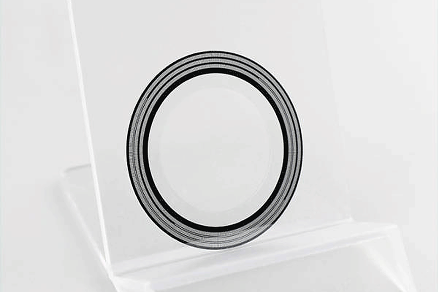
Optical. A light source (usually an infrared LED) shines through a disc etched with alternating transparent and opaque lines; a photodetector counts the transitions. Resolution comes from line density plus electronic subdivision. With quadrature output and a Z index you get an incremental encoder; with a unique code at every angular position you get an absolute one.
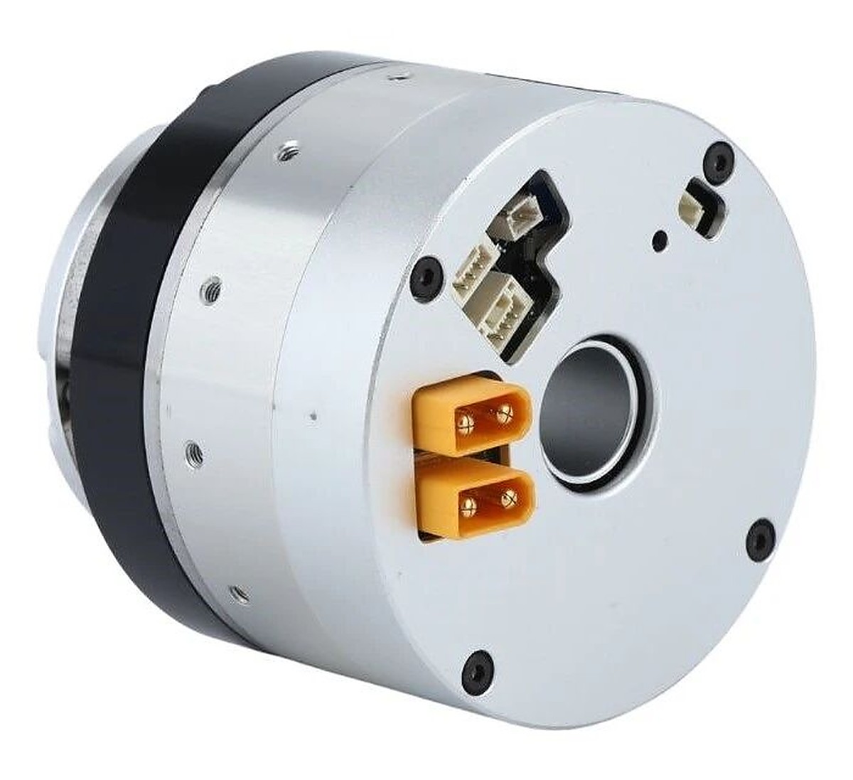
Magnetic. A magnet on the shaft end and a chip on the PCB. The chip — Hall, AMR, GMR or TMR — resolves the field direction into an angle from 0 to 360°. Axial arrangements with a diametrically magnetised magnet tolerate shaft eccentricity best; off-axis arrangements wrap a multi-pole ring around the shaft or the reducer output and read the poles around the circumference, which is what makes a hollow shaft possible.
Inductive. A planar coil is excited with an AC current, establishing an alternating field across the gap; a conductive pattern on the rotor modulates the coupling, and sense windings on the stator output a pair of sine/cosine signals that demodulate to an absolute angle. It is the flat, PCB-wound descendant of the resolver and the inductosyn.
Four consequences follow directly from the physics:
| Optical | Magnetic (chip) | Inductive | |
|---|---|---|---|
| Accuracy ceiling | Highest | Lowest (chip), mid (calibrated ring system) | Mid |
| Contamination | Fails on dust, oil, condensation | Immune | Immune |
| Mounting | Tightest — gap and cleanliness | Smallest, simplest | Flat, large hollow bores |
| Cost structure | System-level | Per chip | System-level |
Optical: the accuracy ceiling, and the maintenance bill
A photoelectric encoder is three things: light source, code disc, photodetector. Two conversions matter in practice:
- Incremental count with quadrature: N = 4 × L, where L is the number of lines on the disc.
- Absolute quantisation step: Δθ = 360° ÷ 2ⁿ, where n is the bit count.
At 25 bits, 2²⁵ = 33,554,432, so the step is about 0.0000107°. Heidenhain’s ECN/EQN 1300 series publishes exactly that order of magnitude: 33,554,432 positions per revolution, accuracy down to ±20 arcsec, maximum operating temperature 115 °C. Tamagawa’s published line-up covers 17-bit and 23-bit single-turn plus multi-turn variants at 23 bits per revolution with 16 bits of turns, and has held the mainstream position in industrial servo for years.
One thing gets lost in the datasheet: resolution is not purely a function of line count. Denser lines mean more expensive disc fabrication and tighter optical alignment, so practical high resolution leans on electronic interpolation of the sine/cosine signals. When evaluating an optical design, read the line count and the output bit count as two separate numbers.
Everything good about optical encoders depends on a clean light path. Dust, oil mist or condensation on the disc degrades the waveform and can drop the square wave entirely — which is why optical feedback on machine tools is fed with sealed, purged air. Three more items belong on the risk list: glass or plastic discs dislike shock and vibration; LEDs age and eventually fail; and some high-resolution variants draw more than 100 mA, which is unwelcome on a battery-powered mobile platform.
Highest accuracy, most mature technology, completely immune to magnetic fields — and an optical system that has to be looked after. Sealing, cleanliness, thermal control and assembly precision each carry a cost.
Magnetic: the chip-ified default
The simplest magnetic encoder is a magnet and one chip. That is also its limitation.
Magnet material decides the thermal behaviour. Samarium-cobalt holds its properties over temperature, neodymium-iron-boron gives the highest energy product in the smallest volume, ferrite is cheap. The neodymium temperature coefficient belongs in the design calculation, not in a footnote:
α(Br) ≈ −0.09% to −0.12% per °C
For multi-pole rings the electrical angle follows θe = p × θm, with p the pole pairs and θm the mechanical angle.
The most common misreading in this category is treating chip resolution as system accuracy. Published numbers make the gap concrete:
| Part | Resolution | System error |
|---|---|---|
| AS5047P | 14-bit | ±0.8° nonlinearity at best installation, up to ±1.2° over temperature and mounting tolerance |
| AS5600 | 12-bit | ±1° typical |
| TLE5012B (GMR) | 15-bit, 0.01° representation | 1.0° maximum over life and temperature with auto-calibration |
| RLS AksIM-2 (off-axis ring system) | up to 20-bit | ±0.004° to ±0.020° after self-calibration, about ±14 to ±72 arcsec |
The first three are “magnetic encoder used as a chip”. The last is “magnetic encoder used as a system” — ring, read head, mounting tolerance and error calibration all designed together. Two orders of magnitude separate them, and the engineering boundary follows: for motor-side commutation and the speed loop, a chip-level part is enough; for output-side position feedback you either design the magnetic circuit as a system — air gap, eccentricity, full-temperature calibration — or move to inductive.
The interference list is unavoidable: motor leakage flux, high-current busbars, nearby ferromagnetic brackets, ring demagnetisation, assembly eccentricity. None of it shows up on a bench demo. It appears in the final structure, the final harness route, at maximum current.
Inductive: flat resolvers, with a size and cost penalty
Inductive encoders measure mutual inductance, not light and not field direction. An excitation coil drives an alternating field across the gap, a rotor pattern modulates the coupling, and stator windings output angle-dependent EMF. Academic reviews describe the inductosyn as “a planar multi-pole resolver”; what modern products do is swap the winding for PCB traces and the analogue demodulation for digital.
That lineage brings specific properties: no light source, so no LED ageing; no permanent magnet, so no remanence drift; planar stator and rotor, so the stack can be thin and light with a large hollow bore.
Zettlex’s production IncOder range illustrates the trade. The 44 mm size offers 10 to 17 bits of resolution at 360 arcsec accuracy; the 70 mm size offers 10 to 20 bits at 125 arcsec; repeatability is 1 LSB. It is insensitive to dust, oil and fingerprints, and meets IEC 61000-6-2 and IEC 61000-6-4 for EMC in the installed state.
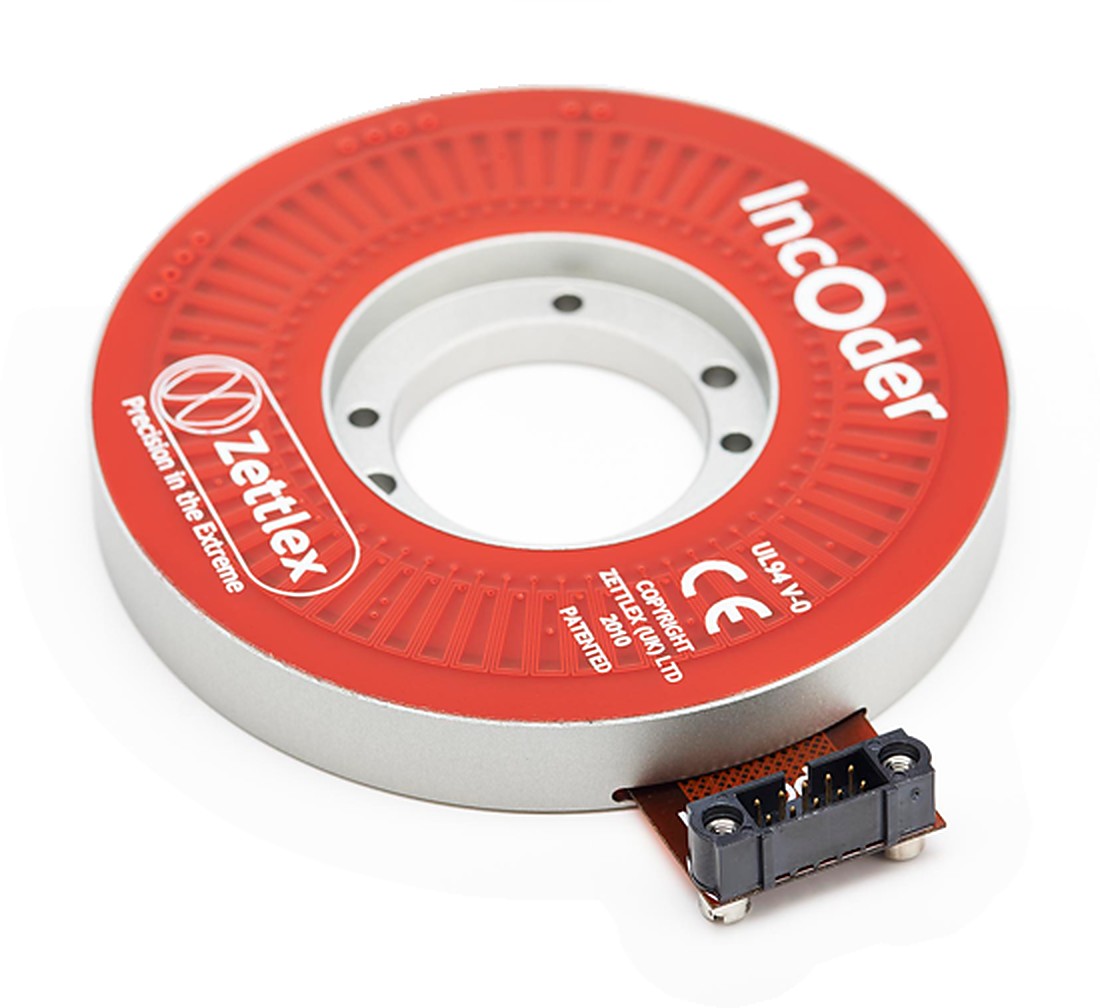
That puts accuracy between chip-level magnetic and high-end optical, with environmental tolerance near magnetic. That combination — robust and reasonably accurate — is the real selling point. The price is explicit: larger diameter than a chip solution, single-unit pricing in the hundreds of dollars on public channels, extra circuit and EMC work for the excitation and demodulation chain, and far fewer suppliers than the other two families.
Where it sits matters more than what it is
Inside one joint, the mounting position decides at least half the performance. This split deserves more attention than the choice between technologies.
Motor side: commutation and the speed loop. The sensor sits on the rotor and measures electrical angle and speed, feeding FOC commutation, the current loop and the speed loop. Resolution requirements are modest; electrical-angle quality is not. A Hall set gives six states per electrical cycle — 60° electrical — enough for block commutation, not enough for high-accuracy FOC. Drive vendor engineering notes put the floor at roughly 500 counts per revolution of incremental signal, or 11-bit single-turn absolute. In practice this position is almost always magnetic: small, tolerant of high speed, cheap, and natural to integrate into the motor.
Output side: seeing backlash and compliance. The output encoder sits after the reducer and measures the true joint angle. Its value is that the motor-side sensor cannot see any of the error the reducer introduces: backlash, flexspline and tooth deflection, bearing and housing compliance. Backlash in common reducers runs 0.3° to 2°, and it happens after the reduction, where motor-side resolution cannot help.
Under an ideal rigid transmission the motor-side step would be divided by the ratio at the output:
Δθ_output ≈ Δθ_motor ÷ N — valid only for a perfectly rigid drive
The problem is precisely that “perfectly rigid” is a property reducers do not have. That is the origin of the familiar result that piling bits onto the motor side does not fix the output.
Dual encoders. Use both: motor side for commutation and the inner speed loop, output side for the outer position loop, with the true joint angle fed directly into the closed loop so transmission error is observed and compensated in real time. Collaborative robots converged on this architecture years ago; UR’s current documentation names it “True Absolute Encoder”.
The difference between the two readings also carries information about torsional deflection, which allows a torque estimate given the equivalent stiffness:
τ_est ≈ Kθ × (θ_motor ÷ N − θ_output)
Be restrained about this one. Harmonic and RV stiffness is nonlinear, friction and hysteresis move with temperature, direction and load, and an uncalibrated estimate is not a substitute for a torque sensor. Treating the dual-encoder difference as an observer of transmission error is closer to engineering reality than treating it as a torque sensor.
Resolution is not accuracy: three numbers to keep apart
- Resolution — the smallest angle the encoder can distinguish, set by bit count and subdivision.
- Accuracy — deviation from the true angle, set by eccentricity, air gap, bearing runout, thermal drift and calibration residual.
- Repeatability — the spread of repeated arrivals at the same position, usually far better than accuracy.
A 20-bit encoder has a quantisation step of 360° ÷ 1,048,576 ≈ 0.000343°. That is the smallest distinguishable step, not the accuracy. Eccentricity, tilt, field non-uniformity, gap variation and bearing runout multiply it by tens or thousands. AksIM-2 is specified at 20 bits with system accuracy starting at ±0.004° for exactly this reason. In the other direction, a 14-bit chip-level magnetic part has a 0.022° step and ±0.8° of mounting nonlinearity — the bit count is irrelevant beside the system error.
The same logic applies to the claim that the reduction ratio “multiplies resolution”. It holds only in ideal kinematics; backlash, mesh error and torsional deflection are outside the formula. What belongs on the datasheet review are system-level accuracy, the error band over temperature, and the mounting tolerance the part demands.
Selection by application
| Application | First choice | Why |
|---|---|---|
| Machine tools, metrology, arc-second servo positioning | Optical absolute | Highest accuracy; the environment can supply sealing, thermal control and assembly precision; also immune to strong magnetic fields |
| Motor-side commutation and speed loop | Chip-level magnetic | Small, cheap, high-speed tolerant, integrates into the motor |
| Reducer output absolute position, hollow shaft | Calibrated magnetic ring or inductive | Accuracy without an optical cavity, and a bore for cabling |
| Oily, dusty plant with mid-level accuracy | Inductive | Contamination-immune with system-level calibration built in |
Five items worth putting on the design review agenda, whichever route is chosen:
- Write requirements as separate line items — absolute accuracy, repeatability, error over temperature, dynamic error, mounting tolerance — not as a single “≥17 bit” clause.
- For magnetic designs, review motor leakage flux, busbar fields, ferromagnetic brackets and magnet drift, and test them in the final structure, final harness and at maximum current.
- For optical designs, review ingress protection, condensation, the shock and vibration spectrum, and disc thermal drift.
- For inductive designs, review air-gap tolerance, the effect of metal structure nearby, the excitation/demodulation chain and system-level EMC.
- For high-ratio joints, prefer output-side absolute feedback or a dual-encoder architecture instead of adding bits on the motor side.
The short version
Encoder selection is the job of finding a reliable physical source for every signal a joint needs. Optical, magnetic and inductive are not ranked; they have boundaries. Light fears contamination, magnetism fears interference, inductive designs care about air gap and the metal around them.
The money-saving insight is that placement dominates part selection. A chip-level magnetic encoder on the motor side plus a calibrated ring or an inductive part on the output side will beat a single expensive optical unit crammed into a joint whose reducer has 1° of backlash — and it will cost less.